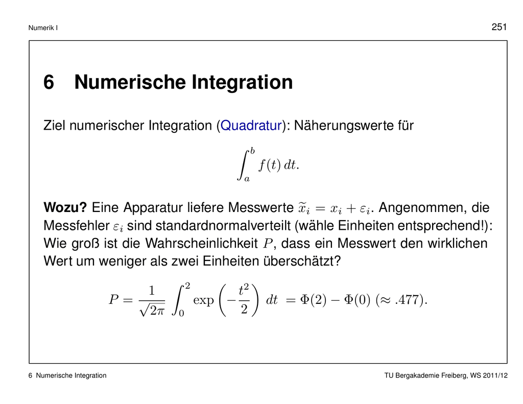
Gauss Quadratur Beispiel
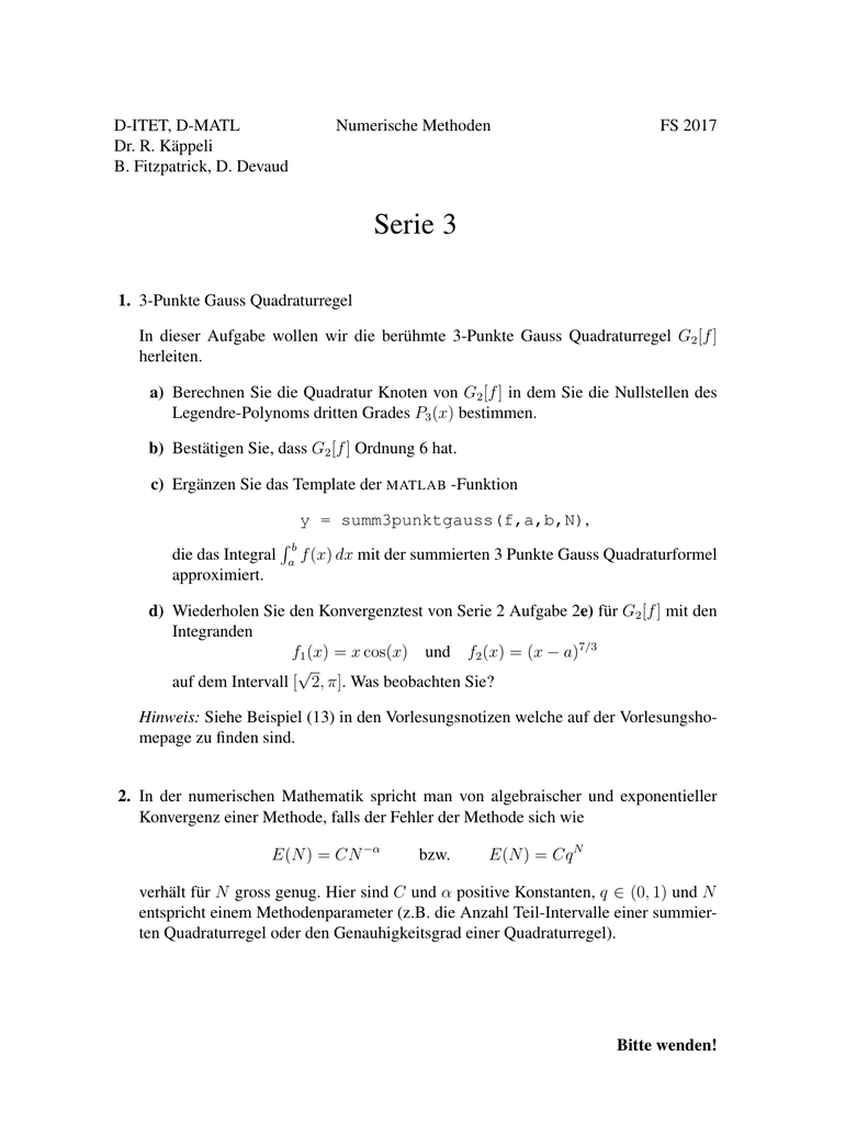


Die gauß quadratur nach carl friedrich gauß ist ein verfahren zur numerischen integration das bei gegebenen freiheitsgraden eine optimale approximation des integrals liefert bei diesem verfahren wird die zu integrierende funktion aufgeteilt in wobei eine gewichtsfunktion ist und durch ein spezielles polynom mit speziell gewählten auswertungspunkten approximiert wird.
Gauss quadratur beispiel. Legendre gauss quadrature is a numerical integration method also called the gaussian quadrature or legendre quadrature. Learn via example how to apply the gauss quadrature formula to estimate definite integrals. A gaussian quadrature over the interval 1 1 with weighting function w x 1. S hj j 1 2.
We simply think about two integrals one in and the other in direction and combine two 1d gq integrations. Wir schlitzen zum schlub noch den einflud der durch corioliskrafte verursachten aber vernachlassigten reibkraft. Gaussian quadrature formulas for the integration of oscillating functions gaussian quadrature formulas for the integration of oscillating functions piessens r. 6 4 gauss sche quadraturformeln beispiel.
0 359140910 t hj j 0 1. I z 1 0 xex x 1 2 dx e 2 2 0 3591409142. Figure 3 3 shows how a sample 4 point gq on a 2d quadrilateral element works. Enjoy the videos and music you love upload original content and share it all with friends family and the world on youtube.
3 3 gauss quadrature integration in 2d gq points and weights for quadrilateral elements are directly related to the ones used for 1d gq. Definition 3 4 8 orthogonalpolynome essei pn n n0 eine folge paarweise orthogonaler po lynomepn pn d h. W x 1 1 x2. Nullstellen xi cos 2i 1 2n 2 π f ur 0 i n des n 1 ten tschebyscheff polynoms tn 1 x cos n 1 arccos x pn 1 f ur x 1 1.
Pi pj ω δij pi pi ω 0 3 25 und exakt vom gradn dannheißendiepn orthogonalpolynome u b e r a b bzgl. Gauß quadratur die gauß quadratur nach carl friedrich gauß ist ein verfahren zur numerischen berechnung von integralen der form a b φ x w x d x int limits a b phi x w x mathrm dx a b φ x w x d x mit optimaler ordnung s unten. For more videos and resources on this topic please visit http. 1970 01 01 00 00 00 kleine ktteilungen ergibt sich fur dieselben phasenportraits auch die darstellung von bild 6b.